Tutorial

Introduction

In this tutorial we will gradually build a complex example that closely mimics a realistic scenario using simulated data. We will pretend to be a bioinformatician involved in a large project for examining de novo mutations in a set of children. We were just given a directory containing the first batch of exome sequence data generated from 100 families comprised of mother, father, and a child and we were asked to examine the quality of the data and to identify de novo substitutions in the 100 children. A de novo substitution is a nucleotide at a given position in a child that is not present in his/her parents at that position.

Setup

snakeobjects and this tutorial are tested and work well on Linux; they don’t work on Windows. We assume that you will work on a Linux or Mac. In addition, we assume that you have conda or miniconda installed (Conda Installation). Everything else needed to follow this tutorial is included in the snakeobjectsTutorial.tgz. When you download and extract (tar xzf snakeobjectsTutorial.tgz) the file, you will get a directory called snakeobjectsTutorial. In the examples that follow we have assumed that the snakeobjectsTutorial directory is created in the /tmp directory, but this is not essential. Everything will work just fine if you have the snakeobjectsTutorial in your home directory or anywhere else.

The snakeobjectsTutorial folder contains one file named environment.yml and two subdirectories: input, and solutions.

The environment.yml file defines the conda environment we will use throughout the tutorial:

name: snakeobjectsTutorial
channels:
  - iossifovlab 
  - bioconda
  - conda-forge
  - defaults
dependencies:
  - snakeobjects
  - pandas
  - matplotlib
  - graphviz

To create the snakeobjectsTutorial environment and to activate it we can use the following commands:

(base) .........................$ cd /tmp/snakeobjectsTutorial
(base) /tmp/snakeobjectsTutorial$ conda env create
(base) /tmp/snakeobjectsTutorial$ conda activate snakeobjectsTutorial
(snakeobjectsTutorial) /tmp/snakeobjectsTutorial$

The command line prompt shows the activated conda environment and the current working directory. We will show this long prompt everywhere below to remind you that you must work under the snakeobjectsTutorial environment and because a lot of the commands depend on the current working directory.

The input directory contains the input data for our project. Inside it you will find a short README.txt file describing the contents. Briefly, the directory contains the reference genome (chrAll.fa), the known genes (genes.txt), and the regions targeted by the exome capture (targetRegions.txt). For the purposes of the tutorial we will use only the first 1MB of human chromosome 1 that contains 54 transcripts from 36 different genes. The genes include 67 protein coding regions/exons that are targeted by the hypothetical exome capture. There are also 768 fastq files in the sub-directories of input/fastq grouped into 384 pairs of read 1—read 2 files (i.e., fastq/FC0A03F0C/L007/bcL_R1.fastq.gz and fastq/FC0A03F0C/L007/bcL_R2.fastq.gz. This is a typical structure of the output for the so-called paired-end sequencing. In addition, there is a file called fastqs.txt providing the additional information for each of the fastq files (i.e., the individuals for each of the fastq files) and the collection.ped file describing the 100 trio families using a standard pedigree file that has one line for each of the 300 individuals.

Finally, the solutions subdirectory contains the state of the pipeline and the projects at various stages (steps) of the tutorial. For example, solutions/step-2.4 contains the state after we have completed Step 2.4. For the impatient, the solutions/final contains the complete pipeline built by the end of the tutorial.

Step 1. Examining the fastq files

We will build a pipeline for achieving our goals or identifying the de novo variants and the judging the quality of the data by small steps. We will start with a simple pipeline that counts the number of pairs of reads for each fastq run.

Step 1.1. Create project and pipeline directories

First, let’s create a directory called pipeline where we will add the pipeline’s components and a directory called project where we will store the results of the pipeline. We will assume that you create these directories in the snakeobjectsTutorial directory:

(snakeobjectsTutorial) /tmp/snakeobjectsTutorial$ mkdir pipeline
(snakeobjectsTutorial) /tmp/snakeobjectsTutorial$ mkdir project

This location of the directories is not required. Provided you are willing to make few minor changes in the projects’ configuration you can create the two directories anywhere.

Step 1.2. Configure the project

Next, we will create a file called so_project.yaml in the project directory with the following content:

so_pipeline: "[D:project]/../pipeline"

inputDir: "[D:project]/../input"
fastqDir: "[PP:inputDir]/fastq"
fastqsFile: "[PP:inputDir]/fastqs.txt"

This so_project.yaml configures our first snakeobjects project. The first line specifies that the pipeline that will operate on this project is contained in the directory ../pipeline relative to the project directory. The [D:project] is an example for interpolation feature available in the project configuration files. Alternatively, we could have specified the pipeline directory using a full path (/tmp/snakeobjectsTutorial/pipeline). The second line adds a configuration property called inputDir that points to the input directory that was given to us. Here we have also used a path relative to the project directory, which is convenient for the purposes of the tutorial. The inputDir parameter will not be used by the pipeline directly. We will only use it in the so_project.yaml file to define the values of other project parameters relative to the inputDir. Indeed, the next two properties fastqsFile and fastqDir are defined succinctly based on the inputDir and point to the table describing the fastq files and to the directory containing the fastq files. Using inputDir is optional — we could have defined the fastqDir as "[D:project]/../input/fastq" or with a full path to the directory, /tmp/snakeobjectsTutorial/input/fastq.

To check if the configuration was successful, we can use the sobjects describe command from within the project directory (the easiest way to tell sobjects which project it should operate on is to ‘go into’ the project’s directory or any of its subdirectories):

(snakeobjectsTutorial) /tmp/snakeobjectsTutorial$ $ cd project
(snakeobjectsTutorial) /tmp/snakeobjectsTutorial/project$ sobjects describe
# WORKING ON PROJECT /tmp/snakeobjectsTutorial/project
# WITH PIPELINE /tmp/snakeobjectsTutorial/pipeline
Project parameters:
    so_pipeline: /tmp/snakeobjectsTutorial/project/../pipeline
    inputDir: /tmp/snakeobjectsTutorial/project/../input
    fastqDir: /tmp/snakeobjectsTutorial/project/../input/fastq
    fastqsFile: /tmp/snakeobjectsTutorial/project/../input/fastqs.txt
Object types:

The result should show that sobjects has determined the project and the pipeline directories and that the fastqDir and fastqsFile project properties point to the correct locations:

....$ head /tmp/snakeobjectsTutorial/project/../input/fastqs.txt
flowcell    lane    barcode individual
FC0A03F09   L006    D       SM90370
FC0B03F03   L001    D       SM90370
FC0A03F09   L006    E       SM03231
FC0B03F03   L001    E       SM03231
FC0A03F09   L006    F       SM79279
FC0B03F03   L001    F       SM79279
FC0A03F0C   L007    D       SM14701
FC0B03F00   L008    D       SM14701
FC0C03F00   L004    D       SM14701

Step 1.3. Create the build_object_graph.py

Now that have configured our first project, we will turn our attention to the pipeline. So far the pipeline directory is empty. The first thing to do when starting a pipeline is to create the build_object_graph.py script. In the Step 1 we will create a very simple graph that contains one object for each fastq pairs of files. The fastq pairs are listed in the fastqs.txt file in the input directory and we have already ensured that our project has a parameter (fastqsFile) that points to the fastqs.txt. The contents of our first build_object_graph.py are shown below. You should create a file named build_object_graph.py in the pipeline directory and copy the shown contents in the file.

import pandas as pd
from pathlib import Path

def run(proj, OG):
    fastqDir = Path(proj.parameters['fastqDir'])
    fastqs = pd.read_table(proj.parameters["fastqsFile"], sep='\t', header=0)

    for i, r in fastqs.iterrows():
        OG.add('fastq', 
                ".".join([r['flowcell'],r['lane'],r['barcode']]),
                {
                    'R1':       fastqDir / r['flowcell'] / r['lane'] / f"bc{r['barcode']}_R1.fastq.gz",
                    'R2':       fastqDir / r['flowcell'] / r['lane'] / f"bc{r['barcode']}_R2.fastq.gz",
                    'sampleId': r['individual']
                }
             )

The run function is given the project (proj) for which it will create a new object graph and object graph instance (OG) that it should add the new objects into. In the first two lines, the function accesses the necessary parameters through proj.parameters: the fastqDir pointing to the directory with the fastq files and the fastqsFile pointing to the table describing the project fastq pairs of files (or fastq runs). The function, then uses pandas to read and iterate over all lines of this table and for each line adds (snakeobjects.ObjectGraph.add()) an object of type fastq and object id equal to the flowcell, lane, and 'barcode properties concatenated with .. For example, the object created for the first line of the fastqs.txt file will have an object id equal to FC0A03F0F.L004.J. Three parameters are also added to each of objects: R1 and R2 point to the fastq files for the first and for the second reads defined relative to the project’s fastqDir parameter, and the sampleId is assigned the value of the individual column.

Step 1.4. Prepare the project

Next we will create the object graph for our project. We do that by using the sobjects prepare command from within the project directory. We can then follow with the sobjects describe to see description of the created object graph:

(snakeobjectsTutorial) /tmp/snakeobjectsTutorial/project$ sobjects prepare
# WORKING ON PROJECT /tmp/snakeobjectsTutorial/project
# WITH PIPELINE /tmp/snakeobjectsTutorial/pipeline
(snakeobjectsTutorial) /tmp/snakeobjectsTutorial/project$ sobjects describe
# WORKING ON PROJECT /tmp/snakeobjectsTutorial/project
# WITH PIPELINE /tmp/snakeobjectsTutorial/pipeline
Project parameters:
    so_pipeline: /tmp/snakeobjectsTutorial/project/../pipeline
    inputDir: /tmp/snakeobjectsTutorial/project/../input
    fastqDir: /tmp/snakeobjectsTutorial/project/../input/fastq
    fastqsFile: /tmp/snakeobjectsTutorial/project/../input/fastqs.txt
Object types:
     fastq : 384

The above says that we have created an object graph that has 384 objects of type fastq, that is exactly what we expected.

Snakemake usually creates paths to all traget files, so there is no need for snakeobjects to create directories for all object types in advance, however snakeobjects creates directories for objects that have symbolic link parameters.

The OG.json file stores the object graph that was just created and the Snakefile is the projects specific snakefile that will be provided to the Snakemake upon execution of the pipeline. In addition, there are directories for each object from the objects graph where the objects’ targets will be stored: the fastq/FC0A03F09.L006.G directory will contain the targets for the object of type fastq and object id FC0A03F09.L006.G. Each of the object directories has also a log subdirectory (i.e., fastq/FC0A03F09.L006.G/log) where log files associated with the object will be stored (more about log files later).

In addition, the sobjects prepare created one file, fastq.snakefile, in pipeline directory. This is not a typical behavior: as a rule, sobjects only updates the project directory, but when we start a new pipeline it’s handy to have placeholders for the object type Snakemake files be created for us. The content if the new fastq.snakefile is very simple:

add_targets()

This simple one line accomplishes nothing but reminding us that the next step would be to declare the targets to be created for objects of type fastq. There is one special target automatically added to every object file, and it is called T("obj.flag"). It is created after all the other targets for the object are successfully created. Without explicitly adding object type targets (as in the current state of the fastq.snakefile), the T("obj.flag") is the only target. We will keep this situation for now, and add useful targets shortly.

Step 1.5. Execute the dummy project

After we have prepared the project, it is time to execute it. This is done by sobjects run command. This command requires at least one argument to that we use to control how to execute the pipeline: -j means that we can use all the available local cores to execute the pipeline (only for snakemake versions before 8.0); -j 1 means that we can use only one of the local cores; -j 2 means that we can use 2 local cores, etc. Alternatively, we can add --profile <cluster profile> option which indicate that we will execute the pipeline by submitting jobs to the computation cluster defined by the <cluster profile>. Executing pipelines on cluster will be covered later. For now, we would use the simplest -j 1 form to execute the dummy pipeline we have developed so far. We can specify more options to the sobjects run command that control the execution of the pipeline and here we would use the -q command that instructs the underlying Snakemake to be ‘quiet’ and produce only minimal output:

(snakeobjectsTutorial) /tmp/snakeobjectsTutorial/project$ sobjects run -j 1 -q
# WORKING ON PROJECT /tmp/snakeobjectsTutorial/project
# WITH PIPELINE /tmp/snakeobjectsTutorial/pipeline
UPDATING ENVIRONMENT:
export SO_PROJECT=/tmp/snakeobjectsTutorial/project
export SO_PIPELINE=/tmp/snakeobjectsTutorial/pipeline
export PATH=$SO_PIPELINE:$PATH
RUNNING: snakemake -s /tmp/snakeobjectsTutorial/pipeline/Snakefile -d /tmp/snakeobjectsTutorial/project -j 1 -q
Job counts:
    count   jobs
    1       so_all_targets
    384     so_fastq_obj
    385

As usual, the first two lines show the project and the pipeline that sobjects operates with. The next five lines provide information about how sobjects executes Snakemake, including the environment variables and the command line parameters passed to Snakemake. Finally, we see the number of successfully executed jobs summarized by the Snakemake rules used for each job. Both rules shown are automatically generated by snakeobjects as indicated by the so_ prefix. The so_all_targets is the default (first) rule Snakemake sees and is the one that specifies all targets that need to be created for the project and is naturally executed only 1 time. The so_fastq_obj rule is used to build an object of type fastq and since we have 384 such objects in our graph this rule is used for 384 jobs.

The sobjects run command added the ./.snakemake directory where Snakemake stored internal information related to the execution. This may come handy for figuring out errors in complex situation but we will not cover the Snakemake privates in this tutorial and refer you to the Snakemake’s documentation for more information. Most importantly, sobjects run created an obj.flag file in directories for each object:

(snakeobjectsTutorial) /tmp/snakeobjectsTutorial/project$ find fastq  | head
fastq
fastq/FC0A03F09.L007.E
fastq/FC0A03F09.L007.E/obj.flag
fastq/FC0A03F0F.L001.D
fastq/FC0A03F0F.L001.D/obj.flag
fastq/FC0B03F00.L005.E
fastq/FC0B03F00.L005.E/obj.flag
fastq/FC0A03F03.L004.D
fastq/FC0A03F03.L004.D/obj.flag
fastq/FC0A03F0F.L003.I

These files represent the T("obj.flag") target and are created only after all of the other targets for the object are created. As we have not yet added any other targets, only the obj.flags are created for the objects.

The pipeline and the project configuration we have developed so far are included in the solutions/step-1.5 directory.

Step 1.6. Add a useful target

Next, we will add an explicit target that does something useful: we will create a target called pairNumber.txt for objects of type fastq that will store the number of paired reads in the fastq object. This is achieved by replacing the auto-generated one line in the pipeline’s fastq.snakemake with the following:

add_targets("pairNumber.txt")

rule countReads:
    input: P('R1'), P('R2')
    output: T("pairNumber.txt")
    run:
        import gzip

        nPairs= 0
        buff = []
        with gzip.open(input[0]) as R1F, \
             gzip.open(input[1]) as R2F:
            for l1,l2 in zip(R1F,R2F):
                buff.append((l1,l2))
                if len(buff) == 4:
                    nPairs += 1
                    buff = []
        
        with open(output[0],"w") as OF:
            OF.write(f'{wildcards.oid}\t{nPairs}\n')

The first line declares that objects of type fastq (the object type is implied by the name of the Snakemake file fastq.snakemake) will have a target named pairNumber.txt.

Next is a Snakemake rule we have called countReads that describes how to create the target: the output clause on line 5 shows that this rule will generate the T("pairNumber.txt") target. As input (line 4), the rule will use the two files pointed by the fastq object’s parameters called R1 and R2. To obtain the value of R1 and R2 parameters for the object the rule uses the extension function P(). These parameters were set so that their values are full file paths to the read 1 and read 2 files within the input/fastq directory for the fastq object.

We use the run clause of the countReads rule to implement the generation of the outputs from inputs by a python snipped. There are alternative clauses that can be used instead of run that allow different ways to implement the output generation (i.e., with shell clause we can use shell commands, like cat, echo to generate the outputs). Later in the tutorial we will demonstrate how to use some of these alternatives.

The python snipped uses the input and output objects provided by Snakemake to access the rule’s input, outputs. The snipped also uses the Snakemake’s object called wildcards object to access the object id (oid) for the object the rule operates on. (For the readers that are familiar with Snakemake, the oid can be explained by the fact that the output: T("pairNumber.txt") is equivalent to output: fastq/{oid}/pairNumber.txt.)

The actual implementation is fairly trivial assuming one knows a bit about the way pair-end sequencing results are represented in the fastq files. Briefly, in pair-end sequencing a small (i.e., 200-500 base-pairs) linear DNA fragments from the genome are sequenced and for each fragment the sequencing machine first reads several (i.e., 100) nucleotides from one side (read 1) of the fragment and several nucleotides from the other end (read 2) of the fragment. The first reads from all fragments are stored in read 1 fastq file and the second reads are stored in the read 2 fastq file. Importantly, the order of the fragments in the read 1 and read 2 fastq files is the same, so that the first read in read 1 fastq files is from the same DNA fragment as the first read in the read 2 fastq file. Reads in a fastq file are represented by 4 consecutive lines (fragment id line, sequence line, separator line, base-quality line).

Step 1.7. Create a test project

We just improved our pipeline to do something useful. In a large project tasks usually take a lot of computational resources and a lot or time. To be able to easily test if the updated pipeline works well it is a good idea to have a test project configured to operate on a small subset of the input data. Here we will do just that. Even though the complete tutorial input data is small enough that the pipeline we have created so far can process it all on a single processor for 2-3 minutes, this is a useful demonstration of how easy it is to maintain and operate on multiple projects with the same snakeobjects pipeline. Moreover, we will extend the pipeline substantially and the final pipeline at the end of the tutorial can take as much as one hour on a single processor to process the full project.

We can create the new projectTest with the following simple commands:

(snakeobjectsTutorial) /tmp/snakeobjectsTutorial/project$ cd ..
(snakeobjectsTutorial) /tmp/snakeobjectsTutorial$ mkdir projectTest
(snakeobjectsTutorial) /tmp/snakeobjectsTutorial$ cd projectTest
(snakeobjectsTutorial) /tmp/snakeobjectsTutorial$ cp ../project/so_project.yaml .
(snakeobjectsTutorial) /tmp/snakeobjectsTutorial$ head -16 ../input/fastqs.txt  > fastqs-small.txt

and replace line 5 in projectTest/so_project.yaml file that configures the fastqsFile project parameter to point to the fastqs-small.txt file containing a description of 15 fastq runs instead of the complete fastqs.txt file with 384 fastq runs:

so_pipeline: "[D:project]/../pipeline"

inputDir: "[D:project]/../input"
fastqDir: "[PP:inputDir]/fastq"
fastqsFile: "[D:project]/fastqs-small.txt"

With the projectTest configured, we can then prepare and run the projects:

(snakeobjectsDev) /tmp/snakeobjectsTutorial/projectTest$ sobjects prepare
# WORKING ON PROJECT /tmp/snakeobjectsTutorial/projectTest
# WITH PIPELINE /tmp/snakeobjectsTutorial/pipeline
(snakeobjectsDev) /tmp/snakeobjectsTutorial/projectTest$ sobjects run -j 1 -q
# WORKING ON PROJECT /tmp/snakeobjectsTutorial/projectTest
# WITH PIPELINE /tmp/snakeobjectsTutorial/pipeline
UPDATING ENVIRONMENT:
export SO_PROJECT=/tmp/snakeobjectsTutorial/projectTest
export SO_PIPELINE=/tmp/snakeobjectsTutorial/pipeline
export PATH=$SO_PIPELINE:$PATH
RUNNING: snakemake -s /tmp/snakeobjectsTutorial/pipeline/Snakefile  -d /tmp/snakeobjectsTutorial/projectTest -j 1 -q
Job counts:
    count   jobs
    15      countReads
    1       so_all_targets
    15      so_fastq_obj
    31
...

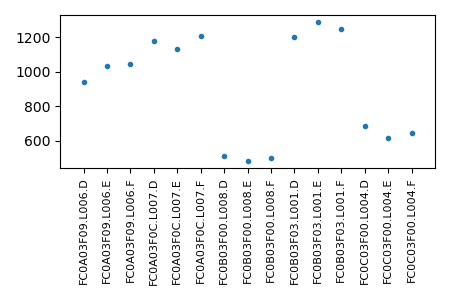
The run finishes almost instantaneously and as a result we can find the pairNumber.txt files for each of the 9 fastq objects created for the projectTest:

(snakeobjectsDev) /tmp/snakeobjectsTutorial/projectTest$ cat fastq/*/pairNumber.txt
FC0A03F09.L006.D    942
FC0A03F09.L006.E    1037
FC0A03F09.L006.F    1048
FC0A03F0C.L007.D    1179
FC0A03F0C.L007.E    1133
FC0A03F0C.L007.F    1206
FC0B03F00.L008.D    511
FC0B03F00.L008.E    483
FC0B03F00.L008.F    502
FC0B03F03.L001.D    1205
FC0B03F03.L001.E    1290
FC0B03F03.L001.F    1251
FC0C03F00.L004.D    684
FC0C03F00.L004.E    614
FC0C03F00.L004.F    647

We can spot check to see if the reported number of reads is correct. For example:

(snakeobjectsDev) /tmp/snakeobjectsTutorial/projectTest$ cat ../input/fastq/FC0A03F09/L006/bcD_R1.fastq.gz | gunzip -c | wc -l
3768

Read 1 file for the fastq run FC0A03F09.L006.D contains 3,768 lines which is equal to 4 times the number of pairs (942) reported in the corresponding pairNumber.txt file. This is exactly what is expected: as described above, sequencing reads are represented in 4 lines in the fastq files.

Step 1.8. Re-run the complete project

Now that have verified that the updated pipeline works, it is time to count the pair numbers for the complete project:

(snakeobjectsDev) /tmp/snakeobjectsTutorial/projectTest$ cd ../project
(snakeobjectsTutorial) /tmp/snakeobjectsTutorial/project$ sobjects run -j 1 -q
# WORKING ON PROJECT /tmp/snakeobjectsTutorial/project
# WITH PIPELINE /tmp/snakeobjectsTutorial/pipeline
UPDATING ENVIRONMENT:
export SO_PROJECT=/tmp/snakeobjectsTutorial/project
export SO_PIPELINE=/tmp/snakeobjectsTutorial/pipeline
export PATH=$SO_PIPELINE:$PATH
RUNNING: snakemake -s /tmp/snakeobjectsTutorial/pipeline/Snakefile -d /tmp/snakeobjectsTutorial/project -j 1 -q
(snakeobjectsTutorial) /tmp/snakeobjectsTutorial/project$ cat fastq/*/pairNumber.txt | head
cat: 'fastq/*/pairNumber.txt': No such file or directory

The results seem strange. Snakemake doesn’t seem to run any jobs and the pairNumber.txt targets are not created. One way to figure out what’s going on is to run Snakemake in verbose mode, by removing the -q flag:

(snakeobjectsDev) /tmp/snakeobjectsTutorial/project$ sobjects run -j 1
# WORKING ON PROJECT /tmp/snakeobjectsTutorial/project
# WITH PIPELINE /tmp/snakeobjectsTutorial/pipeline
UPDATING ENVIRONMENT:
export SO_PROJECT=/tmp/snakeobjectsTutorial/project
export SO_PIPELINE=/tmp/snakeobjectsTutorial/pipeline
export PATH=$SO_PIPELINE:$PATH
RUNNING: snakemake -s /tmp/snakeobjectsTutorial/pipeline/Snakefile -d /tmp/snakeobjectsTutorial/project -j 1
Building DAG of jobs...
Nothing to be done.
Complete log: /tmp/snakeobjectsTutorial/project/.snakemake/log/2021-02-25T114732.563671.snakemake.log

Snakemake says that there is nothing to do. This is a peculiar behavior of Snakemake that manifests anytime we add a new targets and rules to a pipeline and we need to create the new targets in a project that was successfully executed prior to the addition. The way to overcome this is to force Snakemake to create all targets built by the new rule:

(snakeobjectsDev) /tmp/snakeobjectsTutorial/project$ sobjects run -j 1 -R countReads
# WORKING ON PROJECT /tmp/snakeobjectsTutorial/project
# WITH PIPELINE /tmp/snakeobjectsTutorial/pipeline
UPDATING ENVIRONMENT:
export SO_PROJECT=/tmp/snakeobjectsTutorial/project
export SO_PIPELINE=/tmp/snakeobjectsTutorial/pipeline
export PATH=$SO_PIPELINE:$PATH
RUNNING: snakemake -s /tmp/snakeobjectsTutorial/pipeline/Snakefile -d /tmp/snakeobjectsTutorial/project -j 1 -R countReads
Building DAG of jobs...
Using shell: /bin/bash
Provided cores: 192
Rules claiming more threads will be scaled down.
Job counts:
    count   jobs
    384 countReads
    1   so_all_targets
    384 so_fastq_obj
    769
Select jobs to execute...
...

This seems to have done the job and now we do indeed have the pairCount.txt targets:

(snakeobjectsTutorial) /tmp/snakeobjectsTutorial/project$ cat fastq/*/pairNumber.txt | head
FC0A03F00.L001.D    2265
FC0A03F00.L001.E    2181
FC0A03F00.L001.F    2221
FC0A03F00.L001.G    2265
FC0A03F00.L001.H    2170
FC0A03F00.L001.I    2162
FC0A03F00.L002.A    1371
FC0A03F00.L002.B    1276
FC0A03F00.L002.C    1365
FC0A03F00.L002.D    1760
(snakeobjectsTutorial) /tmp/snakeobjectsTutorial/project$ cat fastq/*/pairNumber.txt | wc -l
384

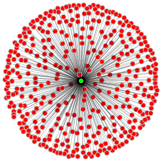
Step 1.9. Add a summary object

It will be convenient to combine all the pairNumber.txt files into one file that can easily be opened in tools like Excel to get a global understanding of the pair counts across all the fastq runs. Such aggregation need is fairly typical in workflows and is easy to implement in snakeobjects. We will add one object in the object graph that will be responsible for aggregating information for all the fastq objects. We typically use xxxSummary as object type and o for the object id of such singleton objects. To add our fastqSummary/o objects we add one line to the build_object_graph.py pipeline script:

import pandas as pd
from pathlib import Path

def run(proj, OG):
    fastqDir = Path(proj.parameters['fastqDir'])
    fastqs = pd.read_table(proj.parameters["fastqsFile"], sep='\t', header=0)

    for i, r in fastqs.iterrows():
        OG.add('fastq', 
                ".".join([r['flowcell'],r['lane'],r['barcode']]),
                {
                    'R1':       fastqDir / r['flowcell'] / r['lane'] / f"bc{r['barcode']}_R1.fastq.gz",
                    'R2':       fastqDir / r['flowcell'] / r['lane'] / f"bc{r['barcode']}_R2.fastq.gz",
                    'sampleId': r['individual']
                }
             )
    OG.add('fastqSummary','o',deps=OG['fastq'])

Importantly, we make the fastqSummary/o object to be dependent by all fastq objects already added to the graph, using the deps=OG['fastq'] parameter. As descried in the snakeobjects.ObjectGraph.__getitem__() method, indexing an objects graph with an object type returns the list of the objects of that type that are in the graph.

We will add two targets to the new fastqSummary object type by creating the fastqSummary.snakefile file in the pipeline directory with the following content:

add_targets("allPairNumbers.txt","pairNumber.png")

rule gatherPairNumbers:
    input:  DT("pairNumber.txt")
    output: T("allPairNumbers.txt")
    shell:  "cat {input} | sort > {output}"

rule pairNumberFigure:
    input: T("allPairNumbers.txt")
    output: T("pairNumber.png")
    run:
        import matplotlib
        matplotlib.use("Agg")
        import pandas as pd 
        import matplotlib.pyplot as plt

        T = pd.read_table(input[0], sep='\t',header=None)

        fig = plt.figure(figsize=(3+len(T)/10, 3))
        plt.plot(T[1],'.')
        plt.xticks(range(len(T)),T[0],rotation=90.,fontsize=8)
        plt.xlim([-1,len(T)])
        plt.tight_layout()
        plt.savefig(output[0])

The first target, called allPairNumers.txt, is created by the gatherPairNumbers rule, as indicated by the output: T("allPairNumbers.txt") clause. This rule for the first time in the tutorial shows the use of one of the most interesting functions of snakeobjects, DT(). The DT() function here specifies that the input of the rule will be the pairNumber.txt targets of the objects the current object depends on. The current object is of type fastqSummary (this is clear by name of the snakefile) and the object graphs generated by our pipeline here is only one object of this type. We made this object to be dependent on the all the fastq objects. Thus, the input for this rule will be all the pairNubmer.txt targets of the fastq objects. The implementation of the rule uses the cat and sort unix tools through the shell clause. The {input} in the implementation is replaced by the list of all pairNumber.txt files related to the pairNumber.txt targets for the fastq objects and the {output} is replaced by the single allPariNumbers.txt output file.

The second target, pairNumber.png is created by the second rule. This target uses the first target as an input and so will be created only after the first one is successfully built. The implementation is in a run clause (a python snipped) that uses matplotlib to draw a simple graph showing all the pair numbers across the fastq objects.

Next, we will re-run our two projects. We will redo the projectTest from scratch to make sure that the complete pipeline functions properly:

(snakeobjectsTutorial) /tmp/snakeobjectsTutorial/project$ cd ../projectTest
(snakeobjectsTutorial) /tmp/snakeobjectsTutorial/projectTest$ sobjects cleanProject -f
(snakeobjectsTutorial) /tmp/snakeobjectsTutorial/projectTest$ sobjects prepare
# WORKING ON PROJECT /tmp/snakeobjectsTutorial/projectTest
# WITH PIPELINE /tmp/snakeobjectsTutorial/pipeline
(snakeobjectsTutorial) /tmp/snakeobjectsTutorial/projectTest$ sobjects run -j 1 -q
# WORKING ON PROJECT /tmp/snakeobjectsTutorial/projectTest
# WITH PIPELINE /tmp/snakeobjectsTutorial/pipeline
UPDATING ENVIRONMENT:
export SO_PROJECT=/tmp/snakeobjectsTutorial/projectTest
export SO_PIPELINE=/tmp/snakeobjectsTutorial/pipeline
export PATH=$SO_PIPELINE:$PATH
RUNNING: snakemake -s /tmp/snakeobjectsTutorial/pipeline/Snakefile -d  /tmp/snakeobjectsTutorial/projectTest -j 1 -q
Job counts:
    count   jobs
    15      countReads
    1       gatherPairNumbers
    1       pairNumberFigure
    1       so_all_targets
    1       so_fastqSummary_obj
    15      so_fastq_obj
    34
....

In the highlighted command we removed OG.json, .snakemake, and all object subdirectories that were created before. This is done with -f option of the command sobjects cleanProject. Thus we lost all previously built targets for the projectTest. So, the sobjects run command then needed to recreate all the targets. For the large project we will only create the new targets:

(snakeobjectsTutorial) /tmp/snakeobjectsTutorial/projectTest$ cd ../project
(snakeobjectsTutorial) /tmp/snakeobjectsTutorial/project$ sobjects prepare
# WORKING ON PROJECT /tmp/snakeobjectsTutorial/project
# WITH PIPELINE /tmp/snakeobjectsTutorial/pipeline
(snakeobjectsTutorial) /tmp/snakeobjectsTutorial/project$ sobjects run -j 1 -q
# WORKING ON PROJECT /tmp/snakeobjectsTutorial/project
# WITH PIPELINE /tmp/snakeobjectsTutorial/pipeline
UPDATING ENVIRONMENT:
export SO_PROJECT=/tmp/snakeobjectsTutorial/project
export SO_PIPELINE=/tmp/snakeobjectsTutorial/pipeline
export PATH=$SO_PIPELINE:$PATH
RUNNING: snakemake -s /tmp/snakeobjectsTutorial/pipeline/Snakefile -d /tmp/snakeobjectsTutorial/project -j 1 -q
Job counts:
    count   jobs
    1       gatherPairNumbers
    1       pairNumberFigure
    1       so_all_targets
    1       so_fastqSummary_obj
    4
    ....

Here we did not remove the objects subdirectory and the targets that were built the last time we executed the pipeline for the large project were preserved. The sobjects prepare command created one new object (the fastqSummary/o) and the sobjects run created its targets. Both the projectTest and project projects now have an aggregated allPairNumbers.txt file (.../fastqSummary/o/allPairNumbers.txt) and a pairNumber.png figure. (...fastqSummary/o/pairNumber.png). The pairNumber.png for projectTest should look like:

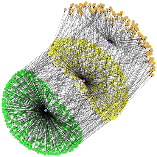
and the pairNumber.png for the large project should look like this:

The large figure is probably not ideal and its layout can be improved. But the birds eye view is informative and its resolution is high enough that one can zoom in enough to see the details.

Step 2. Alignment and target coverage by sample

The most frequent way to use sequence data involves aligning the sequencing reads to a reference genome and the alignment is often the most computationally hard task. Conceptually, alignment is simple. Each read generated by a sequencing machine comes from a random place in the genome of the studied sample. The alignment is the process of finding the location in the reference genome that each read originated from. This can be accomplished if for every read we scored every possible location in the reference genome for how well it matches the given read and if we selected the location that resembled the read best. But genomes tend to be large (i.e., the human genome contains ~3 billion positions) and the number of reads we need to align is also large (i.e., we may have tens or even hundreds of millions of reads for each of tens, hundreds, or thousands of samples we work with). The naive strategy thus fails miserably. Fortunately, there are tools that use powerful indexing approaches and heuristics to find excellent approximations to the optimal alignment and do that fast. We will use the popular bwa tool here.

The next step after alignment is usually finding variants in the samples we study. This involves examining all the reads that overlap every location of interest to identify the nucleotides/alleles at the location, a process known as genotyping. Since the sequencing is noisy and often we study diploid organisms that can have two different alleles in a location, we need to observe many reads for every position in a sample to genotype a position with confidence. If we don’t have enough reads at a position, we are not able to determine the genotypes. An important quality characteristic of the sequence dataset is the distribution of the number of reads covering positions of interest across samples. We refer to this distribution as ‘coverage’ distribution below.

Step 2.1. Reference genome indexing

bwa’s approach to alignment is to create an index for the reference genome. This index is then used to speed up the alignment of the fastq files. We will create an object in our pipeline that will be responsible for the reference genome and for its index:

import pandas as pd
from pathlib import Path

def run(proj, OG):
    fastqDir = Path(proj.parameters['fastqDir'])
    fastqs = pd.read_table(proj.parameters["fastqsFile"], sep='\t', header=0)

    OG.add('reference','o', {'symlink.chrAll.fa':proj.parameters['chrAllFile']})

    for i, r in fastqs.iterrows():
        OG.add('fastq', 
                ".".join([r['flowcell'],r['lane'],r['barcode']]),
                {
                    'R1':       fastqDir / r['flowcell'] / r['lane'] / f"bc{r['barcode']}_R1.fastq.gz",
                    'R2':       fastqDir / r['flowcell'] / r['lane'] / f"bc{r['barcode']}_R2.fastq.gz",
                    'sampleId': r['individual']
                }
             )
    OG.add('fastqSummary','o',deps=OG['fastq'])

The new objects type is reference and its objects id is o as we typically name singleton objects. We set one parameter named symlink.chrAll.fa with a value taken from the project’s parameter chrAllFile. We will add the chrAllFile parameter to our two projects and set it to point to the .../input/chrAll.fa file. We can do that by adding the line chrAllFile: "[PP:inputDir]/chrAll.fa" to the so_project.yaml files of the two projects. (We will assume that you have indeed done that!)

The parameter, symlink.chrAll.fa of our new reference/o object is a special parameter due to its symlink. prefix. Such parameters enable us to create targets for objects during the sobjects prepare phase. When an object has a parameter with name like symlink.L and value P, sobjects prepare will create a symbolic link in the object’s directory called L pointing to the path P. Specifically, our reference object will have a chrAll.fa link (we can think of it as a target) pointing to the ..../input/chrAll.fa. The following commands demonstrate that:

(snakeobjectsTutorial) /tmp/snakeobjectsTutorial/projectTest$ sobjects prepare
# WORKING ON PROJECT /tmp/snakeobjectsTutorial/projectTest
# WITH PIPELINE /tmp/snakeobjectsTutorial/pipeline
(snakeobjectsTutorial) /tmp/snakeobjectsTutorial/projectTest$ ls -l reference/o
total 4
lrwxrwxrwx 1 yamrom   iossifovlab   56 Feb  8 12:04 chrAll.fa -> /tmp/snakeobjectsTutorial/projectTest/../input/chrAll.fa

We will add one target to the reference object type by copying the following in the pipeline/reference.snakefile file:

add_targets("chrAll.bwaIndex.flag")

rule makeBwaIndex:
    input: T("chrAll.fa")
    output: touch(T("chrAll.bwaIndex.flag"))
    conda: "env-bwa.yaml"
    resources: mem_mb=10*1024
    log: **LFS("bwa_index")
    shell: "(time bwa index {input} -a bwtsw > {log.O} 2> {log.E} ) 2> {log.T}"

This small rule uses many snakeobjects/Snakemake features for the first time in the tutorial. First, the input clause refers to the T("chrAll.fa") target built at the prepare phase through the symlink. parameter we discussed just above. Second, the output for the rule is a ‘flag’ target/file that is created with the touch function. This construct is very convenient when the rule produces multiple files or has multiple steps and we want to indicate that all the rule is supposed to do is done. Snakemake’s touch function creates (or updates the time-stamp of) such files upon successful execution of its shell (or run, or script) clause. In our case, we use the bwa index command that generates several files next to the reference genome fasta (.fa) file.

Third, the makeBwaIndex rule uses a conda clause, indicating that the rule should be executed with a different conda environment than the one we run sobjects in. The conda clause’s argument (env-bwa.yaml) points to a file that describes the new environment to be created for this rule. We usually place such files in pipeline directory and in this case we add the following content to the .../pipeline/env-bwa.yaml file:

channels:
  - bioconda
dependencies:
  - samtools 
  - bwakit

The bwakit is the conda package that contains the bwa tool and the samtools is a tool that is used to manipulate the bam files that store the alignment results generated by bwa. We will re-use the same environment in different rules that directly use samtools shortly. In this case we could have easily added bwa and samtools to our global environment (snakeobjectsTutorial/environment.yml file), but it often happens that we cannot build one environment that has all the tools necessary for all rules in a pipeline because the rules may have contradictory requirements. For example, two rules may require two different versions of the same tool, or rules may use tools that depend on different version of the python. Such conflicts are easily handled by allowing different environments for different rules. Unfortunately, the conda clauses are not used by default and we need to explicitly provide a --use-conda parameter to Snakemake. We will show how to do that through sobjects run shortly.

Forth, we added the resources clause. This clause enables us to let Snakemake know what the resource needs are to execute the given rule. Indexing of the small reference genome provided with the tutorial does not need large amounts of memory but indexing the complete human genome with bwa uses 10Gb. Declaring the required resources for each rule that uses a lot is particularly important when we run sobjects or Snakemake on a computational cluster, where job scheduling and monitoring are guided by such requirements.

Fifth, the rule uses Snakemake’s log clause together with snakeobjects’ convenience function LFS() to configure log files where we can store information about the execution of the rule. The LFS() function configures three log files associated with the object the rule operates on and stored into the object’s log directory. The three log files are: log.O typically used for standard output, log.E used for standard error, and log.T used for timing measures. The names for these log files are <log name>-out.txt, <log name>-err.txt , and <log name>-time.txt, respectively, where the <log name> is the parameter given to the LFS() function. For example, the log.O from our makeBwaIndex rule for the projectTest project is: /tmp/snakeobjectsTutorial/projectTest/reference/o/log/bwa_index-out.txt To actually create the bwa index for our projects, we need to execute sobjects run. But to convince Snakemake to notice the conda clauses, we have to provide the --use-conda command line argument: (snakeobjectsTutorial) /tmp/snakeobjectsTutorial/projectTest$ sobjects run -j --use-conda. Moreover, we have to provide this option every time we do sobjects run in the future when we extend the pipeline or when we process new data. snakeobjects provides a better solution. We can define a project parameter called default_snakemake_args whose value is a set of command line parameters passed to Snakemake automatically every time we do sobjects run. To take advantage of that we will add the line default_snakemake_args: "--use-conda" to so_project.yaml files for both of our projects. For example, after we have added the default_snakemake_args and the chrAllfile parameters, the so_project.yaml file for the projectTest should look like:

so_pipeline: "[D:project]/../pipeline"
default_snakemake_args: "--use-conda"

inputDir: "[D:project]/../input"
fastqDir: "[PP:inputDir]/fastq"
fastqsFile: "[D:project]/fastqs-small.txt"
chrAllFile: "[PP:inputDir]/chrAll.fa"

Now let’s run the sobjects run and examine the results:

(snakeobjectsTutorial) /tmp/snakeobjectsTutorial/projectTest$ sobjects run -j 1
# WORKING ON PROJECT /tmp/snakeobjectsTutorial/projectTest
# WITH PIPELINE /tmp/snakeobjectsTutorial/pipeline
UPDATING ENVIRONMENT:
export SO_PROJECT=/tmp/snakeobjectsTutorial/projectTest
export SO_PIPELINE=/tmp/snakeobjectsTutorial/pipeline
export PATH=$SO_PIPELINE:$PATH
RUNNING: snakemake -s /tmp/snakeobjectsTutorial/pipeline/Snakefile -d /tmp/snakeobjectsTutorial/projectTest --use-conda -j 1
Building DAG of jobs...
Creating conda environment /tmp/snakeobjectsTutorial/pipeline/env-bwa.yaml...
Downloading and installing remote packages.
Environment for ../../pipeline/env-bwa.yaml created (location: .snakemake/conda/b244435f)
Using shell: /bin/bash
Provided cores: 192
Rules claiming more threads will be scaled down.
Job counts:
    count   jobs
    1       makeBwaIndex
    1       so_all_targets
    1       so_reference_obj
    3
Select jobs to execute...
...

(snakeobjectsTutorial) /tmp/snakeobjectsTutorial/projectTest$ ls -l reference/o/*
-rw-r--r-- 1 yamrom iossifovlab       0 Feb 27 17:13 reference/o/chrAll.bwaIndex.flag
lrwxrwxrwx 1 yamrom iossifovlab      56 Feb  8 12:04 reference/o/chrAll.fa -> /tmp/snakeobjectsTutorial/projectTest/../input/chrAll.fa
-rw-r--r-- 1 yamrom iossifovlab      67 Feb 27 17:13 reference/o/chrAll.fa.amb
-rw-r--r-- 1 yamrom iossifovlab     138 Feb 27 17:13 reference/o/chrAll.fa.ann
-rw-r--r-- 1 yamrom iossifovlab 1000116 Feb 27 17:13 reference/o/chrAll.fa.bwt
-rw-r--r-- 1 yamrom iossifovlab  250007 Feb 27 17:13 reference/o/chrAll.fa.pac
-rw-r--r-- 1 yamrom iossifovlab  500064 Feb 27 17:13 reference/o/chrAll.fa.sa
-rw-r--r-- 1 yamrom iossifovlab       0 Feb 27 17:13 reference/o/obj.flag

reference/o/log:
total 8
-rw-r--r-- 1 yamrom iossifovlab 494 Feb 27 17:13 bwa_index-err.txt
-rw-r--r-- 1 yamrom iossifovlab   0 Feb 27 17:12 bwa_index-out.txt
-rw-r--r-- 1 yamrom iossifovlab  42 Feb 27 17:13 bwa_index-time.txt
(snakeobjectsTutorial) /tmp/snakeobjectsTutorial/projectTest$ cat reference/o/log/bwa_index-time.txt

real        0m0.633s
user        0m0.508s
sys 0m0.021s

The first highlighted line shows that the --use-conda parameter was indeed passed to Snakemake even though we did not explicitly provide it on the command line. The second highlighted line shows the message from Snakemake that it is building a conda environment based on the env-bwa.yaml file. Finally, the list of the reference/o directory shows that the chrAll.bwaIndex.flag was created together with the five files (chrAll.fa.amb, chrAll.fa.ann, chrAll.fa.bwt, chrAll.fa.pac, and chrAll.fa.sa), that contain the bwa index. The list also shows the three log files that were created and the last command shows the content of the bwa_index-time.txt one that tells us that took 0.633s to create this index.

Step 2.2. Alignment of fastq

With the bwa reference genome index created, it is time to align the reads in our fastq runs. We will store the alignments as a target of the fastq objects that have already been added to the object graph, but since the alignment uses the reference genome index will make the fastq objects to be dependent on the reference/o object. This is easily accomplished by a small change (adding the highlighted line) in the pipeline’s build_objects_graph.py script:

import pandas as pd
from pathlib import Path

def run(proj, OG):
    fastqDir = Path(proj.parameters['fastqDir'])
    fastqs = pd.read_table(proj.parameters["fastqsFile"], sep='\t', header=0)

    OG.add('reference','o', {'symlink.chrAll.fa':proj.parameters['chrAllFile']})

    for i, r in fastqs.iterrows():
        OG.add('fastq', 
                ".".join([r['flowcell'],r['lane'],r['barcode']]),
                {
                    'R1':       fastqDir / r['flowcell'] / r['lane'] / f"bc{r['barcode']}_R1.fastq.gz",
                    'R2':       fastqDir / r['flowcell'] / r['lane'] / f"bc{r['barcode']}_R2.fastq.gz",
                    'sampleId': r['individual']
                },
                OG['reference']
             )
    OG.add('fastqSummary','o',deps=OG['fastq'])

We will add the new target (fastq.bam) and the rule that creates it to the end of our pipeline/fastq.snakefile file:

add_targets("pairNumber.txt")

rule countReads:
    input: P('R1'), P('R2')
    output: T("pairNumber.txt")
    run:
        import gzip

        nPairs= 0
        buff = []
        with gzip.open(input[0]) as R1F, \
             gzip.open(input[1]) as R2F:
            for l1,l2 in zip(R1F,R2F):
                buff.append((l1,l2))
                if len(buff) == 4:
                    nPairs += 1
                    buff = []
        
        with open(output[0],"w") as OF:
            OF.write(f'{wildcards.oid}\t{nPairs}\n')

add_targets("fastq.bam")

rule align:
    input:
        refFile       = DT("chrAll.fa"),
        refFileBwaIdx = DT("chrAll.bwaIndex.flag"),
        R1File        = P("R1"),
        R2File        = P("R2")
    output:
        T("fastq.bam")
    params:
        sId = P('sampleId')
    conda: "env-bwa.yaml"
    resources: 
        mem_mb = 5*1024
    threads: 5
    log: **LFS('align')    
    shell:
        "(time bwa mem -t {threads} -R '@RG\\tID:{wildcards.oid}\\tSM:{params.sId}' \
                       {input.refFile} {input.R1File} {input.R2File} 2> {log.E} |   \
               samtools view -Sb - > {output}                                       \
         ) 2> {log.T}"

The new target, fastq.bam, is a bam file. bam is a well-accepted binary file standard format for storing the results of alignments. sam files are the text version of the bam files. The bwa tool we use for alignment generates sam format that is easily converted into the more efficient bam format using samtools. That is the reason we required samtools to be part of the env-bwa.yaml conda environment which we here re-use in our new align rule. In the new rule, we avoid storing the large sam files by piping (|) the sam output of bwa through samtools and storing only the significantly smaller bam files.

The align rule demonstrates a couple of important snakeobjects/Snakemake features. For the first time in this rule we use named inputs. The rule has four inputs, and we have called them refFile, refFileBwaIndex, R1File, and R2File. Named inputs can be used in the implementation of the rule using constructs like {input.refFile}. This clearly improves the readability compared to {input[0]} particularly in rules with many inputs of different types. It’s worthwhile pointing out that the refFileBwaIndex is listed as an input but is not explicitly used in the implementation. Snakemake will execute this rule only after all its inputs have been created which is important here because bwa implicitly requires the index files that must have been prepared before the chrAll.bwaIndex.flag is created. The refFile and refFileBwaIndex are set to point to the chrAll.fa and chrAll.bwaIndex.flag targets of the dependency reference/o object, while R1File and R2File are taken for the current object’s parameters R1 and R2.

Also, for the first time, the align rule shows Snakemake’s params and threads clauses. The params clause allows each execution of the rule to be tuned by use of rule specific parameters. With snakeobjects we often set the rule’s parameters with values taken from parameters of the object the rule operates on (i.e., P()) or from global project parameters (PP()). The parameters of the rule can then be used in the implementation of the rule using constructs like {params.sId}. The threads clause is the way to inform Snakemake of the number of threads the rule will use in its implementation. Alignment of sequencing reads with bwa is a task that can benefit greatly from the use of threads. The tool typically loads into memory a fairly large index and then uses that index to align tens or even hundreds of millions of reads or read pairs. Each read is aligned independently. Having many threads share the same index but process different reads goes a long way towards optimizing memory usage, a resource that is frequently a bottleneck in large sequence analysis projects. But when we execute on computational cluster we have to take into account the number of cores configured on the individual cluster nodes and how easy it is to schedule a job requiring many threads in typical cluster loads or when we run large projects. The ability to control the number of threads, memory, and other resources separately for each rule makes is possible to develop a strategy for balancing the many conflicting requirements.

We will now create the alignment bam files first for the projectsTest project and then for the large project. We need to recreate the object graph (by running sobjects prepare) because we introduced the new dependence of fastq objects on the reference/o. But unless we start from scratch, by removing the object's directories, we would need to help Snakemake a bit by asking explicitly to run the align rule—here we are again in the situation when we add a target to an already complete object.

(snakeobjectsTutorial) /tmp/snakeobjectsTutorial/projectTest$ sobjects prepare
(snakeobjectsTutorial) /tmp/snakeobjectsTutorial/projectTest$ sobjects run -j 1 -R align
# WORKING ON PROJECT /tmp/snakeobjectsTutorial/projectTest
# WITH PIPELINE /tmp/snakeobjectsTutorial/pipeline
UPDATING ENVIRONMENT:
export SO_PROJECT=/tmp/snakeobjectsTutorial/projectTest
export SO_PIPELINE=/tmp/snakeobjectsTutorial/pipeline
export PATH=$SO_PIPELINE:$PATH
RUNNING: snakemake -s /tmp/snakeobjectsTutorial/pipeline/Snakefile -d /tmp/snakeobjectsTutorial/projectTest --use-conda -j 1 -R align
Building DAG of jobs...
Using shell: /bin/bash
Provided cores: 192
Rules claiming more threads will be scaled down.
Job counts:
    count   jobs
    15      align
    1       so_all_targets
    1       so_fastqSummary_obj
    15      so_fastq_obj
    32
Select jobs to execute...
...

On the small projectTest this finishes quickly, well under a minute. But when you repeat the same commands for the large project (we expect that you will indeed to that) it may take several minutes to create all 384 alignment files. And in real sequence alignment projects it is impractical to run many alignments on a single computer. One of the most important features of snakeobjects, directly inherited from Snakemake, is that the same pipeline without any change can be executed on a computational cluster by simply providing the command line parameter --profile=<cluster profile> to the sobjects run. The <cluster profile> points to a directory that contains the setup necessary to submit jobs on a given cluster. The configuration of the cluster profiles is beyond the scope of this tutorial publicly available profiles and descriptions can be found here). If you happen to have one available or, if go through the steps described in Working with clusters, you should by all means execute the tutorial pipelines on your cluster. Note though that the jobs generated by running the tutorial projects are all small because we prepared a toy input datasets. For small jobs like these the overhead of submitting and scheduling may be unnecessarily large. When you get a cluster profile configured, you may also consider adding the --profile=<cluster profile> to the default_snakemake_args project parameter. Every time that you use sobjects run for that project the Snakemake will submit jobs to the cluster instead of running them locally on your computer as it does when you pass the -j 1 option.

Step 2.3. Target coverage by sample and globally

In this step we will introduce two new object types, sample and sampleSummary. The sample object type will be the most complicated object type in this tutorial but will introduce only few of the snakeobjects’ features. The point of this step is to demonstrate how the functionality introduced so far is powerful enough to implement a fairly complex part of the pipeline.

A sample object will represent all sequence data for one individual. We did not pay much attention until now, but sampleId parameter of the fastq objects specifies the sample (or individual) whose genome is represented in the sequence reads in the fastq files. If you examine the input/fastqs.txt file, you will see that some individuals have one fastq run, but others have two or three fastq runs.

It is important to verify if we have enough sequencing reads for each sample. One way to check if the number of reads is ‘enough’ is to examine the distribution of the number of reads covering the positions of interest (or coverage). In our project, the positions of interest are represented by the targetRegions.txt file in the input directory. To measure the coverage (and to be able to identify de novo variants later) it is convenient to merge all the fastq bam files for an individual into a single sample bam file. Then, we can use the single file to examine the depth (number of covering reads) for all the positions in the target regions. Once we have the coverage for every position in the target and for every sample, we can compute statistics of the depth per sample, and visualize the coverage distribution per sample and globally across all samples.

To implement this plan, we will add a project parameter called target that points to the input/targetRegions.bed file to the so_project.yaml for our two projects. For example, the projectTest/so_project.yaml should look like that after the addition of the highlighted line:

so_pipeline: "[D:project]/../pipeline"
default_snakemake_args: "--use-conda"

inputDir: "[D:project]/../input"
fastqDir: "[PP:inputDir]/fastq"
fastqsFile: "[D:project]/fastqs-small.txt"
chrAllFile: "[PP:inputDir]/chrAll.fa"
target: "[PP:inputDir]/targetRegions.bed"

We will then update the build_object_graph.py script in our pipeline by adding a few lines (highlighted below) that create the sample objects referenced by the fastq objects already added to the object graph:

import pandas as pd
from pathlib import Path
from collections import defaultdict

def run(proj, OG):
    fastqDir = Path(proj.parameters['fastqDir'])
    fastqs = pd.read_table(proj.parameters["fastqsFile"], sep='\t', header=0)

    OG.add('reference','o', {'symlink.chrAll.fa':proj.parameters['chrAllFile']})

    for i, r in fastqs.iterrows():
        OG.add('fastq', 
                ".".join([r['flowcell'],r['lane'],r['barcode']]),
                {
                    'R1':       fastqDir / r['flowcell'] / r['lane'] / f"bc{r['barcode']}_R1.fastq.gz",
                    'R2':       fastqDir / r['flowcell'] / r['lane'] / f"bc{r['barcode']}_R2.fastq.gz",
                    'sampleId': r['individual']
                },
                OG['reference']
             )
    OG.add('fastqSummary','o',deps=OG['fastq'])

    sampleFastqOs = defaultdict(list)
    for o in OG['fastq']:
        sampleFastqOs[o.params['sampleId']].append(o) 
    for smId,fqOs in sampleFastqOs.items():
        OG.add('sample',smId,deps=fqOs)

    OG.add('sampleSummary','o',deps=OG['sample'])
    

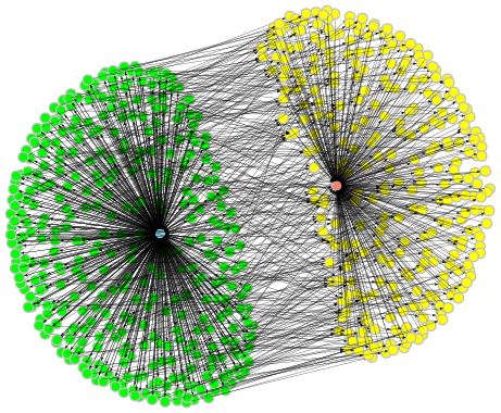
The code above is simple enough (assuming one knows basic python). But the resulting graph becomes non-trivial. Before the addition of the sample object, there were two dependency types: (1) all fastq objects depended on the single reference/o object and (2) the single fastqSummary/o object depended on all fastq objects. Each sample object is dependent only on the one, two, or three fastq objects that are related to this sample, breaking the one-to-all dependence types. At the last line we also add the singleton sampleSummary/o object that will be responsible for aggregating statistics from all sample objects.

We will add six targets for the objects of type sample. The target definition, their relationships, and rules that create them are shown below and you should copy the following content to a file called sample.snakefile within the pipeline directory.

add_targets("sample.bam", "sample.bam.bai","markDupStats.txt")

rule merge:
    input: DT("fastq.bam")
    output: temp(T("raw.bam"))
    conda: "env-bwa.yaml"
    log: **LFS('merge')
    shell: "(time samtools merge -n {output} {input} > {log.O} 2> {log.E} ) 2> {log.T}"

rule reorganizedBam:
    input: T("raw.bam"), DT("chrAll.fa",level=2)
    output: T("sample.bam"), T("markDupStats.txt")
    conda: "env-bwa.yaml"
    log: **LFS('reorganize')
    shell: '''
        (time 
            samtools fixmate -m --reference {input[1]} -O bam {input[0]} - |
            samtools sort -T {input[0]} -O bam | 
            samtools markdup -T {input[0]} -O bam -s --reference {input[1]} - {output[0]} 2> {output[1]}
        ) 2> {log.T}
    '''

rule indexBam:
    input: T("sample.bam")
    output: T("sample.bam.bai")
    conda: "env-bwa.yaml"
    log: **LFS('merge')
    shell: "(time samtools index -b {input} {output} > {log.O} 2> {log.E} ) 2> {log.T}" 

add_targets("depth.txt","coverage-stats.txt","coverage.png")

rule targetDepth:
    input:
        bam=T("sample.bam"),
        idx=T("sample.bam.bai")
    output: T("depth.txt")
    params: target=PP("target")
    conda: "env-bwa.yaml"
    log: **LFS('targetDepth')
    shell: "(time samtools depth -b {params.target} -a {input.bam} > {output} 2> {log.E}) 2> {log.T}"

rule coverageStats:
    input: T("depth.txt")
    output: T("coverage-stats.txt")
    run:
        import pandas as pd 
        D = pd.read_table(input[0], sep='\t',header=None)[2]
        coverageStr = ['%.1f' % (100*sum(D[D >= k])/sum(D)) for k in [1,10,20,40]]
        with open(output[0],"w") as OF:
            OF.write(f'{wildcards.oid}\t' + "\t".join(coverageStr) + "\n")

rule coverage:
    input: T("depth.txt")
    output: T("coverage.png")
    run:
        import matplotlib
        matplotlib.use("Agg")
        import pandas as pd 
        import matplotlib.pyplot as plt

        D = pd.read_table(input[0], sep='\t',header=None)[2]
        coverage = [100*sum(D[D >= k])/sum(D) for k in range(41)]
        fig = plt.figure(figsize=(5, 3))
        plt.plot(coverage,'b.-')
        plt.grid(1)
        xtcks = range(0,41,5)
        plt.xticks(xtcks, [f'{d}x' for d in xtcks])
        plt.xlim([0,40])
        ytcks = range(0,101,20)
        plt.yticks(ytcks, [f'{p}%' for p in ytcks])
        plt.ylim([0,100])
        plt.ylabel('percent of the target covered at >= X')
        plt.title(f"Coverage for sample {wildcards.oid}")
        plt.tight_layout()
        plt.savefig(output[0])

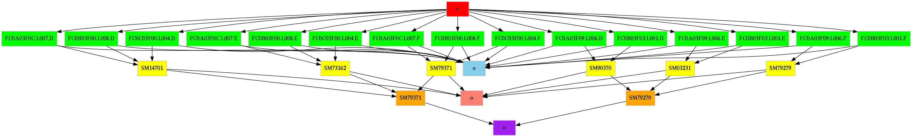
The six targets are related in a complex within-object and across-object target dependencies represented by the input and output clauses of the rules. In addition, to the six targets the sample.snakefile uses a temporary target T("raw.bam"). It is declared as temporary using Snakemake’s function temp. Temporary targets are created as normal targets but are removed when all the downstream rules that use them finish successfully. The DT() function, enables us to concisely define across-objects target dependencies. The figure below, shows a graphical representation of the target dependency relationship of the targets of one of the sample objects overlaid on top of the object-graph dependency relationships.

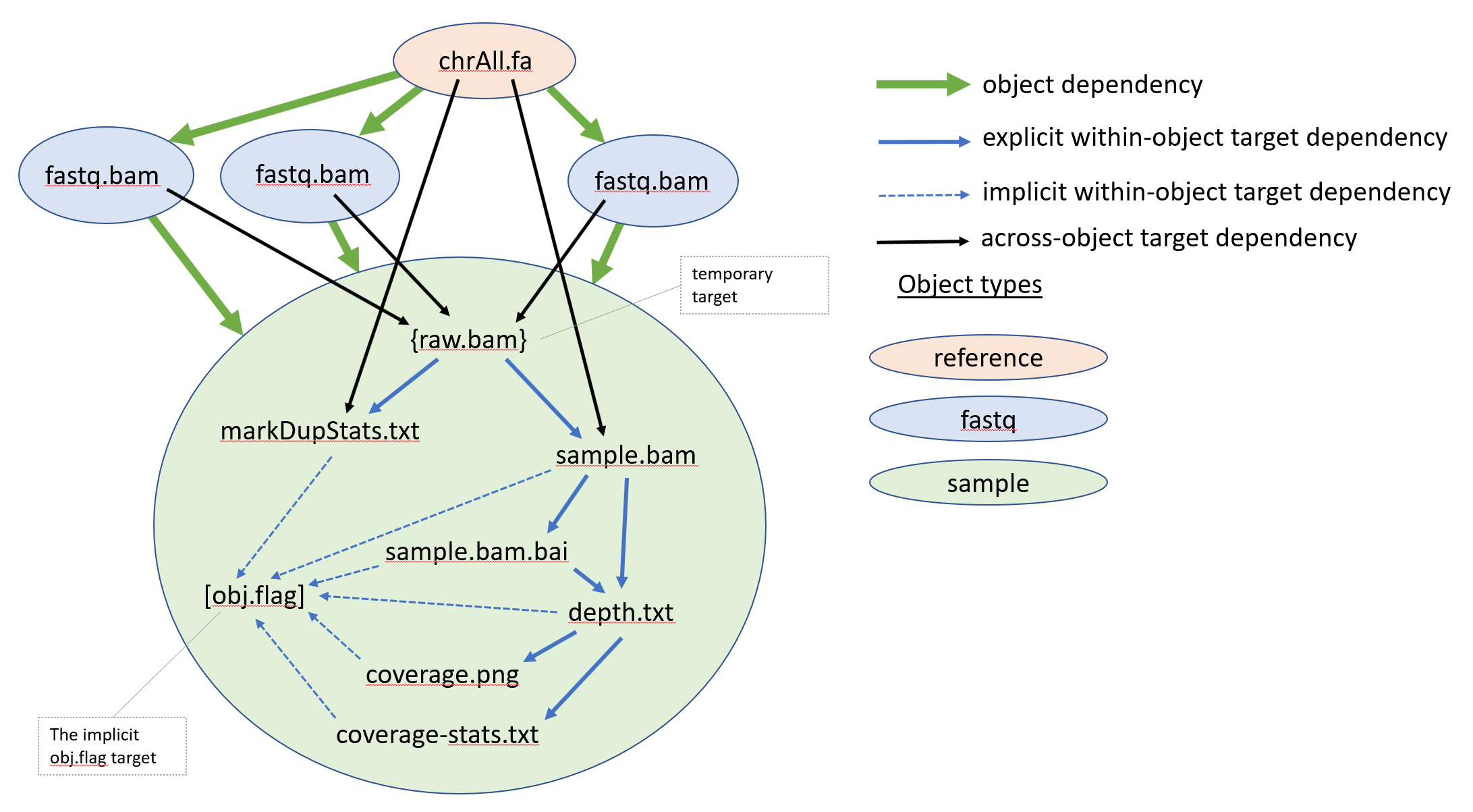
We want to point out two interesting features used in the sample.snakefile. The first one is the level=2 parameter passed on the DT() function call in the rule normalizedBam. It means that we are referring to targets in objects that are two steps away in the object graph. In the specific case, the implementation of the rule requires the chrAll.fa file that is stored as a target of the reference/o object. The sample objects do not depend directly on the reference/o object in our graph, but they depend on one or more fastq objects which in turn depend on the reference/o. Thus, reference/o is ‘two steps’ away in the object graph from the sample objects. The second feature is that a rule can create more than one output targets, as our reorganizedBam rule does.

For each sample, we first merge the related fastq.bam files in one bam file called raw.bam using the samtools merge command. Then we go through a process of ‘cleaning up` the raw.bam file by a series of commands well accepted in the sequence analysis field (fixmate, sort, markdup). The implementation of the reorganizedBam rule uses piping extensively, an approach that saves the expensive writes/reads to disk if we saved the intermediate files. The markdup step identifies read pairs that appear to be duplicates of each other, flags the duplicates, and saves the updated bam file. In addition, markdup writes statistics, like the number of duplicate reads identified, on its standard error. The reorganizedBam rule captures this stream and saves it in the markDupStats.txt target. The percent of duplicated reads in bam file is an important quality measure that one should pay attention to. To avoid getting this tutorial even longer, we do not discuss the markDupStats.txt further. The main output of the reorganziedBam rule is the cleaned, flagged, and sorted (by genomic coordinates) sample.bam file. We next create an index sample.bam.bai for the sample.bam file that allows quick access to the reads aligned at a given genomic region. This index is used to measure the depth for every position in our target regions in the depth rule that saves the resulting depths in the depths.txt target file. Finally, for each sample, we use the depths.txt (1) to create a figure (coverage.png) showing the distribution of the depths and (2) to record the percent of the target positions covered by at least 1, 10, 20, and 40 reads in the coverage-stats.txt target. The coverage.png and the coverage-stats.txt are created by two separate rules, both of which use depths.txt and are implemented by small python snipped using a run: clause.

To finish the updates to the pipeline you should copy the content bellow to the sampleSummary.snakefile in our pipeline:

add_targets("allCoverageStats.txt","allCoverages.png")

rule gatherCoverageStats:
    input:  DT("coverage-stats.txt")
    output: T("allCoverageStats.txt")
    shell:  "cat {input} | sort -k4n > {output}"

rule allCoveragesFigure:
    input: T("allCoverageStats.txt")
    output: T("allCoverages.png")
    run:
        import matplotlib
        matplotlib.use("Agg")
        import pandas as pd 
        import matplotlib.pyplot as plt

        T = pd.read_table(input[0], sep='\t',header=None)

        fig = plt.figure(figsize=(3+len(T)/10, 3))
        plt.plot(T[1],'.',label='X >= 1')
        plt.plot(T[2],'.',label='X >= 10')
        plt.plot(T[3],'.',label='X >= 20')
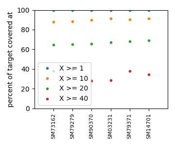
        plt.plot(T[4],'.',label='X >= 40')

        plt.xticks(range(len(T)),T[0],rotation=90.,fontsize=8)
        plt.xlim([-1,len(T)])
        plt.ylim([0,100])
        plt.ylabel('percent of target covered at')
        plt.legend(loc='lower left')
        plt.tight_layout()
        plt.savefig(output[0])

sampleSummary objects has two targets. The first one is called allCoveratStats.txt and its implementation aggregates the coverage-stats.txt from all the sample objects and sorts by the percent of the target covered by at least 20 reads (the 4th column in the coverage-stats.txt files). The second target, called allCoverages.png, is a figure showing the coverage statistics across all samples.

By now, it should be clear how execute the updated pipeline for the two projects: change the working directory to the project directory; do sobjects prepare (we need to run prepare because we updated the build_object_graph.py script and we need to create a new object graph); do sobjects run -j 1.

Once you have successfully run the two projects you should have a figure like

for each sample. The objects/sampleSummary/o/allCoverages.png for the projectTest and for the large project should look like:

Step 3. Calling de novo variants

To finish the tutorial, we will implement a quick and dirty de novo caller and will integrate it into our pipeline. Our de novo caller will look for de novo nucleotides found in children that are not present in their parents. Its implementation is shown below:

#!/usr/bin/env python

import pysam,sys
import pandas as pd
import numpy as np
from collections import Counter,defaultdict

dadBamF,momBamF,chlBamF,targetFile = sys.argv[1:]

AFS = [pysam.AlignmentFile(bmf) for bmf in [dadBamF,momBamF,chlBamF]]
smIds = [ {x['SM'] for x in AF.header['RG']}.pop() for AF in AFS ]

print("\t".join([f'{p}Id' for p in ['dad','mom','chl']] + ['chrom','pos','newAllele'] + 
                [f'{p}.{a}' for p in ['dad','mom','chl'] for a in "ACGT"]))
TT = pd.read_table(targetFile, sep='\t',names=['chr','beg','end'])
for ri,rgn in TT.iterrows():
    cntBuff = defaultdict(list)
    for AF in AFS:
        plps = AF.pileup(rgn['chr'],rgn['beg'],rgn['end'])
        for plp in plps:
            cnt = Counter([n.upper() for n in plp.get_query_sequences()])
            cntA = np.array([cnt[n]  for n in 'ACGT'])
            cntBuff[plp.reference_pos].append(cntA)
    for pos,cntAs in cntBuff.items():
        if len(cntAs) != 3: continue
        trioCnt = np.vstack(cntAs)
        dpths = trioCnt.sum(axis=1)
        for dnvAlleleCandidate in range(4):
            if trioCnt[2,dnvAlleleCandidate] >= 3 and \
               trioCnt[0,dnvAlleleCandidate] == 0 and \
               trioCnt[1,dnvAlleleCandidate] == 0 and \
               dpths[0] >= 10 and dpths[1] >= 10:
                print("\t".join(map(str,smIds + [rgn['chr'], pos,"ACGT"[dnvAlleleCandidate]] + 
                                        list(trioCnt.flatten()))))
for AF in AFS: AF.close()

It is implemented in python and you should copy the above in a file called call_denovo.py in our pipeline directory and make sure that it is flagged as executable (chmod +x call_denovo.py. The only quality this implementation has is that it is short. Otherwise, it is a poorly coded (although not impossible, it will be a challenge for one to understand it), and performs poorly. But it would do for the purposes of the tutorial. Those of you who actually care about finding de novo variants should improve this implementation substantially or, even better, replace it all together with a ‘proper’ de novo caller.

The call_denovo.py is a command line scripts that expects four arguments: the bam files for the father, for the mother, for a child and a list of target regions that contain the positions in which the script will search for de novo alleles. The script uses the popular python module pysam that provides access to reads stored in bam files. The pysam is neither included in our global environment nor in the env-bwa.yaml one. We thus crate a new environment env-pysam.yaml that requires the pysam package. You should copy the following in the env-pysam.yaml file in our pipeline directory— we will use it shortly. The env-pysam.yaml environment requires two additional packages, numpy and pandas, used by the call_denovo.py script.

channels:
  - bioconda
dependencies:
  - pysam
  - numpy
  - pandas

The call_denovo.py script iterates over all the regions in the targetFile and counts the number of reads supporting each of the four nucleotides, A, C, G, and T at every position within the current region. For positions that are covered by reads in the three bam files (see the mysterious line 25), the script checks if there are de novo alleles. A de novo allele is reported if all of the following criteria are met:

• the allele is seen in 3 or more reads in the child (line 29);

• the allele is NOT seen in either of the parents (lines 30 and 31);

• both parents have at least 10 reads covering the positions (line 32).

To integrate the call_denovo.py script in the pipeline, we will create two new objects types, trio and trioSummary. The trio object will represent a father, a mother, and a child trio. In our project the family relationships are described in the input/collection.ped file. The top 10 lines of the file are shown below:

familyId  personId  fatherId  motherId  sex       affected
F0        SM07279   .         .         F         0
F0        SM04710   .         .         M         0
F0        SM63089   SM07279   SM04710   M         ?
F1        SM18469   .         .         F         0
F1        SM64466   .         .         M         0
F1        SM78901   SM18469   SM64466   F         ?
F2        SM88283   .         .         F         0
F2        SM91580   .         .         M         0
F2        SM19841   SM88283   SM91580   M         ?

The question marks in the affected column indicate that the affected status of the children is ‘masked’. This can be done in real projects to avoid bias in the handling between the cases and controls.

We will use the collections.ped file in the build_object_graph.py pipeline script to create the trio objects. As already done multiple times, we will add a project parameter (pedigree) in our two projects that points to the collection.ped file. After the addition, the so_project.yaml file for the projectTest looks like:

so_pipeline: "[D:project]/../pipeline"
default_snakemake_args: "--use-conda"

inputDir: "[D:project]/../input"
fastqDir: "[PP:inputDir]/fastq"
fastqsFile: "[D:project]/fastqs-small.txt"
chrAllFile: "[PP:inputDir]/chrAll.fa"
target: "[PP:inputDir]/targetRegions.bed"
pedigree: "[PP:inputDir]/collection.ped"

The additions the build_object_graph.py are highlighted bellow:

import pandas as pd
from pathlib import Path
from collections import defaultdict

def run(proj, OG):
    fastqDir = Path(proj.parameters['fastqDir'])
    fastqs = pd.read_table(proj.parameters["fastqsFile"], sep='\t', header=0)

    OG.add('reference','o', {'symlink.chrAll.fa':proj.parameters['chrAllFile']})

    for i, r in fastqs.iterrows():
        OG.add('fastq', 
                ".".join([r['flowcell'],r['lane'],r['barcode']]),
                {
                    'R1':       fastqDir / r['flowcell'] / r['lane'] / f"bc{r['barcode']}_R1.fastq.gz",
                    'R2':       fastqDir / r['flowcell'] / r['lane'] / f"bc{r['barcode']}_R2.fastq.gz",
                    'sampleId': r['individual']
                },
                OG['reference']
             )
    OG.add('fastqSummary','o',deps=OG['fastq'])

    sampleFastqOs = defaultdict(list)
    for o in OG['fastq']:
        sampleFastqOs[o.params['sampleId']].append(o) 
    for smId,fqOs in sampleFastqOs.items():
        OG.add('sample',smId,deps=fqOs)

    OG.add('sampleSummary','o',deps=OG['sample'])

    ped = pd.read_table(proj.parameters["pedigree"], sep='\t', header=0)
    for i, r in ped.iterrows():
        if r['fatherId'] == '.' or r['motherId'] == '.': continue
        if not set([r['fatherId'],r['motherId'],r['personId']]).issubset(set(sampleFastqOs)): continue
        OG.add('trio',r['personId'], {"familyId":r['familyId'],"sex":r['sex'],"affected":r['affected'] }, [
                    OG['sample',r['fatherId']],
                    OG['sample',r['motherId']],
                    OG['sample',r['personId']]
                ])
    OG.add('trioSummary','o',deps=OG['trio'])
    

The script will create trio objects only for the children described in the pedigree file (line 33) and only for the children for which the sample objects for the father, for the mother, and for the child have already been created in the object graph (line 34). The object id for the trio objects will be set to the sampleId (called personId in the pedigree file) of the child and the newly created trio are made dependent on the samples for the father, mother, and child. A very important feature of snakeobjects is that the order of the dependencies is preserved in the object graph. The implementation for the single target of the trio objects depends on this order: father’s sample, mother’s sample, child’s sample. See the content bellow and copy it into the new trio.snakefile file in the pipeline directory:

add_targets("denovo_calls.txt")

rule callDenovos:
  input:
    bams=DT("sample.bam"),
    idx=DT("sample.bam.bai")
  output: T("denovo_calls.txt")
  conda: "env-pysam.yaml"
  params:
    bed = PP("target")
  log: **LFS("denovo_calls")
  shell:
    "(time call_denovo.py {input.bams} {params.bed} > {output} 2>{log.E}) 2> {log.T}"

In the highlighted line, the DT("sample.bam") will return a list of 3 bam files, with the first one being the sample.bam file for the father, the second one being the sample.bam file for the mother, and the third one being the sample.bam file for the child, honoring the order in which the object dependencies were listed in the creation of the trio object.

Apart from the important issue about the dependency order, the callDenovos rule demonstrates the use the function PP() to access a project parameter in the configuration of the rule’s parameters.

Finally, the trioSummary.snakefile is also fairly simple, and contains one target, allDenovoCalls.txt, that is the union of the de novo variants found in the individual trios:

add_targets("allDenovoCalls.txt")

rule gatherDenovos:
    input: DT("denovo_calls.txt")
    output: T("allDenovoCalls.txt")
    shell: '''
        head -1 {input[0]} > {output}
        for t in {input}; do
            tail -n +2 $t >> {output}
        done
        '''

One useful trick in the trioSummary.snakefile is the way we use the shell commands head, for, and tail, to combine several files that have identical header, without repeating the header multiple times.

We can now re-run the project, and projectTest with sobjects prepare and sobjects run. Below, we show the .../projectTest/trioSummary/o/allDenovoCalls.txt after the execution of the projectTest is done (and with a bit of manual formatting in Excel):

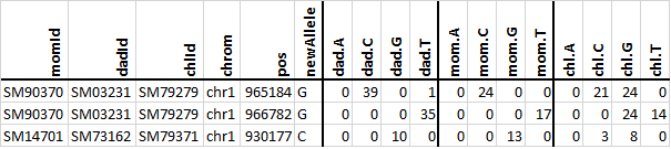
Two de novo variants are identified in the SM79279 child and one is identified in the SM79371 child. The first de novo is an G allele at position chr1:965184 that is: supported by 24 reads (which is larger than 3) in the child; not seen at all in his parents (dad.G and mom.G are both 0) and both parents have more than 10 reads covering the chr1:965184 position (dad has 39 + 1 = 40 reads and mom has 24 reads). All the criteria for a de novo allele are thus met. All the criteria are also met for the other two reported de novo variants. But, the third variant (the new C at chr1:930177) just barely meets the cut-offs and it is possible that it is a false de novo call–the three C s in the child may all be due to noise, or a C in one of the parents may have failed to get sampled in the few reads from that location.

When you successfully execute the large project, you should get a list of 47 de novo variants.

Summary

Congratulations to all of you who are reading this sentence! This was an objectively very long tutorial. For a bit of fun at the end, we will use the sobjects graph command to create a visual summary of the many steps for both of small projectTest and the large projects.

(snakeobjectsTutorial) .................$ cd /tmp/snakeobjectsTutorial/solutions
(snakeobjectsTutorial) /tmp/snakeobjectsTutorial/solutions$ for s in step-1.8 step-1.9 step-2.1 step-2.2 step-2.3 final; do
    (cd $s/projectTest; sobjects prepare;
     sobjects graph -t oId -s box -l lgnd.dot | dot -Tpng > g.png;
     cat lgnd.dot | dot -Tpng > lgnd.png);
done
(snakeobjectsTutorial) /tmp/snakeobjectsTutorial/solutions$ for s in step-1.8 step-1.9 step-2.1 step-2.2 step-2.3 final; do
    (cd $s/project; sobjects prepare;
     sobjects graph -w 0.1 -p 0.2 -a 0.2 | neato -Tpng > g.png);
done

step	projectTest	project	object type
1.8
1.9
2.1
2.2
2.3
3.0